A walk-through basic statistical analyses in Excel, with a causality aim

(0). Preliminaries

0.i. What is ‘scientific research’?

*** Simply: a systematic discovery process that follows agreed-upon methodology and verification rules. Practically: understanding the natural (and more) world, deriving the ‘laws’ that govern it (or law-like rules[i]).

There are many ‘sciences’ out there[ii], and the community of researchers advancing each of their fields, sometimes radically change their approach (paradigm shifts, Kuhn, e.g.).

The ‘scientific method’ in general has been extensively investigated; three such less-known Herculean efforts are worth noting: Bernard Bolzano [3] in 1837, Alfred Korsybski [4] in 1933, and James Fetzer [1] in 1981.

0.ii. What is research methodology?

*** Each science has slightly different such methods or procedures for arriving at agreed-upon truths; philosophy has its own research methodology too, for instance [5] [iii].

‘Research design’ belongs to the ‘research methodology’ package, and it means the specific procedure for measurement and collection of data, analysis and interpretation (‘inferring truths’). Health research, clinical research, and public health research have slightly different emphases, but share largely some elements, like: measurement/instrument development; validity and reliability; analysis of data and causal inference.

0.iii. How does statistics/data analytics mix in the research methodology equation?

(A). Variables are mainly of two kinds: categorical (‘this’ vs. ‘not this’) or continuous (e.g. 29.5, one’s BMI, Body Mass Index)[iv]: the math differs broadly between the two[v], and there are other variants (counts of ‘this’, e.g.), but modern stats can handle them easily (not always intuitively though, see ‘logistic regression’: entire textbooks are devoted to this analytic model, for good reasons).

We skip for now the ‘types of data’ that health and clinical researchers extract and investigate, but just note that some comes from within organs, i.e. investigating molecular-level dynamical processes, other within-person still but ‘lots if it’ (‘big data’), like genetic data, or brain imaging, some more ripe for between-person RQs, like BMI, while other data come in from higher levels, like regional epidemiologic data: sometimes we are called to combine them, and ask more complex RQs, and use more complex statistics (multi-level models, e.g.).

(i). Because people differ so much, and on so many levels, the ‘typical’ value of a variable is a useful practical ‘tool’ in modeling health relevant processes: formally it is called the ‘expected value’, but the ‘mean’[vi] is a more common label. The intuition is quicker (while simplifying!) visually: ‘averaging’ is a form of ‘fitting’ values in a simpler shape: if some have low BMI values, some high values, the average value comes from inquiring: ‘what if all had the same value (but the total would be the same), what would that be’? Van Inwagen’s example shows just that[vii].

(ii). At its core, statistics is merely a process of counting ‘ducks’[viii], and comparing totals, of and between the ‘same’ things[ix]. Practically, however, analyses handle two types of variables:

(1). Categorical, of which the yes/no (1/0) binary kind is the main one, all the other one s(like ‘racial group’) being reduceable to as many binary ones as categories (e.g. White/no, Black/no, etc);

(2). Continuous, like BMI or A1C or Systolic blood pressure (SysBP).

(iii). Statistical tests answer Research Questions (RQs), and absent RQs are uninformative with respect to data: they, by themselves, do not ‘make sense of data’. So let’s take some 1 by 1, btw, all are implanted in Excel, posted @ Tinyurl.com/101STATSEXCEL

***Statistics quick intro accompanying the Youtube walkthroughs.

(1). First from 1. Tinyurl.com/INTRSTATS1

RQ.1. Research Question 1: Are there more overweight males than females?

*** The RQ invites relating 2 binary variables, and the chi-squared test is implemented by hand in the worksheet: it simply compares 4 values, crossing the 2 levels of each binary variable, so how many cases are in each cross-categories (0,0), (1,0), (0,1), and (1,1), to another such set of 4 numbers, the 4 n’s in the null-hypothesis (H0) setup of ‘independence’, or formally P(Overweight | Gender) = P(Overweight), meaning gender does not add information in predicting if one is overweight (in the expected context); this translates directly in the same % of overweight in the males as in the females group. Note that the cells  (0,0) and (1,1) indicate the presence of a ‘relation’, same in one variable goes hand in hand with same in the other, while (1,0) and (0,1)point to lack of a relationship, high in one go hand in hand with ‘low’ in the other one. Note also that chi-squared test is non-directional, it does not tell us which (if!) causes the other one…

*** This asks whether these conditional (on gender, knowing gender, ‘fixing’ gender by ‘seeing’ it, not by intervention!, not ‘setting’ it) probabilities are equal

P(Overweight | Males) P(Overweight | Females)

RQ.1.b. Research Question 1: Do males and females differ in body mass?

*** This asks us to compare some average BMI levels, of males and females, so it asks (if we use Expectation(BMI) for Average(BMI)) to compare these averages (conditional on gender, knowing it, ‘fixing’ it by ‘seeing’ it)

E(BMI | Males) E(BMI | Females)

*** A plain t-test for independent samples would answer this quite well, but many statistical tools can ‘hammer this nail’: a regression of BMI on ‘female gender’ (=1, or ‘yes’) would yield as a conditional mean (called ‘intercept’ in regression modeling, a bit confusing) the value E(BMI | Males), and the regression coefficient would tell us how much higher (if >0) or lower (if<0) is the BMI for females.

RQ.2. Research Question 2: Do patients change their BMI category (overweight vs. not) pre to post?

*** This illustrates how a same 2by2 cross-table can be read completely differently: the 4 inside cells (0,0), (1,0), (0,1), and (1,1) now mean something else (than the chi-squared test example in RQ.1.):  (0,0) and (1,1) mean stability=no change, whereas (1,0) and (0,1) mean changes (up, and down). So the H0 changes its context and setup: it means stability, or expects no cases in the (1,0) and (0,1) cells. It also points to a possible alternative test, by creating a ‘change score’.

RQ.2.b. Research Question 2: Do patients change their BMI levels?

*** This can be answered by a simple ‘related samples’ t-test, which is in fact a ‘model of change’, of which we can use better ones (see [14] or URL)

(2). Then from Tinyurl.com/INTRSTATS2

RQ.3. Is the level of HgA1c predicted by BMI?

*** This implements by hand a simple regression analysis, of one continuous (‘dependent’, we assign this status) variable unto another continuous variable (‘independent’, improperly called, it is not truly not dependent on anything). Excel can run such an analysis with its free ‘Data Analysis’ add-on.

RQ.4.: What is the effect of BMI on Systolic Blood Pressure (BP)?

*** This prepares us for the 3 continuous variables models to follow; it’s just like RQ.3.

(3). Then from Tinyurl.com/INTRSTATS4

RQ.4.a.: What is the effect of BMI on Systolic Blood Pressure (BP), net of (distinct from) that of A1c?

*** This is now a multiple regression analysis, also implemented by hand, to illustrate how the initial effect’ seen RQ.4. changes, and why: when the 2 predictors are themselves co-related, this change will always happen.

RQ.4.b.: Does the direct effect of BMI on Systolic Blood Pressure (BP), vary with the level of HgA1c?

*** This is a natural extension of the RQ.4.a. above, because if there is such ‘effect modification’, we cannot really speak of ‘an’ effect of BMI, but a range of such effects,

RQ.4.c.: What is the total effect of BMI on Systolic Blood Pressure (BP), including the indirect effect through HgA1c?

*** This RQ steps us out of the regression modeling domain, and allows for one variable to be both a predictor/cause and an outcome/effect: the mediator is such a variable. This changes the logic drastically: we do not speak of just one direct effect of BMI, but a larger one, which has a direct and an indirect pathways into the final outcome: the RQ itsels contains this word in it, for this reason (some are interested in the indirect effect only ‘Is A1c mediation the effect of …?’)

RQ.4.d.: Does the indirect effect of BMI on Systolic Blood Pressure (BP), through HgA1c, vary with the very level of BMI?

*** This is a simple extension similar to the move from multiple regression to multiple regression with interaction; now we step into what is improperly perhaps called ‘causal’ mediation: such a model can be easily analyzed, it can be done ‘by hand’ too (I recommend intuitive graphical freeware Onyx, e.g.). More details here [15] or at URL.

RQ.5.:Is there a common cause (latent factor, e.g. “Bad Health”) behind all 3: BMI, HgA1c, and Systolic BP?

*** This illustrates how simple it is to ‘run a factor analysis by hand’ in Excel: the factor loadings are calculated using the ‘tracing rule’ shown in part 3 here. It shows that latent variables’ are just variables themselves, we just don’t have the data for them in the datasets!

RQ.6. Research Question: Are cases changing over 3 time points similarly? (Are those starting off higher changing slower?)

*** This similarly shows how one can derive variances and the covariance between two latent variables, also by hand (but replicated in Onyx)

(4). And then the spatial analytics example from  Tinyurl.com/INTRSTATS3 with Tinyurl.com/BLOGSTATS3 Excel @ Tinyurl.com/SPATIALSSM

RQ.7.: Are states with more residents in poverty expected to live shorter lives? By how much, cmparing classic vs. spatial regression?

*** This implements in Excel for the first time (I think) a spatial regression: extending a regression, done by hand, to account for the interdependencies (‘nonindependence’, ‘autocorrelation’) present in spatial )areal, regional) data. More details here [16] or at URL.

*** Other such walk-throughs are within reach, e.g. for survival analysis, and such.

***I will show in part 3 several tools to derive causal effects from non-interventional or observational data.

References

1. Fetzer, J.H., Scientific knowledge: Causation, explanation, and corroboration. Vol. 69. 1981: Springer Science & Business Media.
2. Munson, R., Why medicine cannot be a science. The Journal of Medicine and Philosophy, 1981. 6(2): p. 183-208.
3. Bolzano, B., Theory of science (Wissenschaftslehre). 1837 (2014).
4. Korsybski, A., Science and sanity An introduction to Non-Aristotelian Systems. 1933, New York: Science Press Printing Co.
5. Williamson, T., Philosophical Method: A Very Short Introduction. 2020: Oxford University Press.
6. Bandyopadhyay, P.S. and M.R. Forster, Philosophy of Statistics, ed. D.M. Gabbay, P. Thagard, and J. Woods. Vol. 7. 2011: Elsevier.
7. Albert, J.B. and A.J. Rossman, Workshop Statistics: Discovery with Data. A Bayesian approach. 2001: John Wiley & Sons.
8. Hoffman, L., Longitudinal analysis: Modeling within-person fluctuation and change. 2015: Routledge.
9. Devore, J.L., Probability and statistics for Engineering and the Sciences. Pacific Grove: Brooks/Cole, 2016.
10. Inwagen, P.v., The Rev’d Mr Bayes and the Life Everlasting, in Reason and Faith: Themes from Richard Swinburne, M. Bergmann and J.E. Brower, Editors. 2016, Oxford University Press. p. 196-219.
11. Conover, W.J., Practical nonparametric statistics. Food and Agriculture Organization of the United Nations. 1999, New York: Willey & Sons.
12. Roughgarden, J., Theory of population genetics and evolutionary ecology: an introduction. 1979.
13. Fetzer, J.H., Sociobiology and epistemology. Vol. 180. 1985: Springer Science & Business Media.
14. Coman, E.N., et al., The paired t-test as a simple latent change score model. Frontiers in Quantitative Psychology and Measurement, 2013. 4, Article 738.
15. Coman, E.N., F. Thoemmes, and J. Fifield, Commentary: Causal Effects in Mediation Modeling: An Introduction with Applications to Latent Variables https://pmc.ncbi.nlm.nih.gov/articles/PMC5298993/. Frontiers in Psychology, 2017. 8(151).
16. Coman, E.N., S. Steinbach, and G. Cao, Spatial Perspectives in Family Health Research https://pubmed.ncbi.nlm.nih.gov/34910138/ https://academic.oup.com/fampra/article/39/3/556/6463006. Family Practice, 2022. 39(3): p. 556–56.

Footnotes:

[i] Example of formal treatment of such options: “Let us differentiate terminologically between lawlike sentences (whether subjunctive or causal conditional in form) and instantiations of sentences of this kind by referring to the latter as “nomological conditionals” (of either subjunctive or causal conditional form). We may further distinguish the two kinds of nomological conditionals as “simple” and as “causal”, respectively.

It obviously follows that lawlike sentences are completely general nomological conditionals, i.e., all nomological conditionals are instantiations of lawlike sentences. It also follows (less obviously, perhaps) that nomic conditionals of neither kind are logically true, since the lawlike sentences which they instantiate attribute permanent properties to the members of reference classes, where the possession of those properties is never implied by the descriptions

of those classes.” [1] p. 49.

[ii] How many ‘sciences’ are there? Is ‘implementation science’ a science? ‘Communications science’? ‘Exercise Science’? Ask Claude.ai. e.g. [see Appendix]. There are also ‘memory science’, ‘learning science’, and … the science of ‘cause and effect’ (or ‘causal inference’, see Pearl’s BoW p. 10: ‘not a fancy name’).

– Sciences can be thought of as ‘physical sciences, life sciences, and Earth sciences’, or on another dimension ‘Social Sciences, Formal Sciences, and Applied Sciences’.  Medicine e.g. belongs to life sciences and is an applied science (some questioned its membership among sciences, see [2], published in The Journal of Medicine and Philosophy!

Another ordering dimension can be ‘how causal their theories’, or how strong causal statements and predictions a science makes, or using alternative language how much uncertainty, unexplained ‘data’, or ‘model error’ component each science carries.

* “Medicine can, of course, be scientific in ways that are easily specified, and medicine can participate in scientific research and contribute to scientific understanding.” & “science and medicine are inherently different.”  & “medicine and science differ both in their aims and their criteria for success: the aim of medicine is to promote health through the prevention and treatment of disease, while the aim of science is to acquire knowledge; medicine judges its cognitive formulations by their practical results in promoting health, while  science evaluates its theories by the criterion of truth.” & “medicine (as  medical practice) has a moral aspect that is not present in science”).

[iii] Philosophers have been involved in serious statistical matters too for a long while, especially in the causality domain; but there is also Philosophy of statistics [6], which has a chapter on ‘Various Issues about Causal Inference’ for instance, but also on ‘Approaches to Simplicity Related to Inference and Truth’ and on ‘Attempts to Understand Different Aspects of “Randomness” ’.

[iv] i. “In this book, we will distinguish between two different types of variables. A categorical variable is a characteristic of an individual which can be broken down into different classes or categories.

Simple examples of a categorical variable are the eye color of a student, the political affiliation of a voter, the manufacturer of your current car, and the letter grade in a particular class.

Typically, a categorical variable is nonnumerical, although numbers are occasionally used in classification.

The social security number of a person is an example of a categorical variable, since its main purpose is to identify or classify individuals. Binary variables are categorical variables for which only two possible categories exist.

A measurement variable is a number associated with an individual that is obtained by means of some measurement. Examples of a measurement variable include your age, your height, the weight of your car, and the distance that you traveled during your Thanksgiving vacation. A measurement variable will have a range of possible numerical values. A person’s age, for example, ranges from 0 to approximately 100.” [7]  p. 5

1. “Throughout the text, I will use the phrase continuous for quantitative variables (even if they are not truly continuous in the sense of having all possible intermediate values between integers), and the phrase categorical for discrete, grouping variables (i.e., in which differences between specific levels are of interest, although those levels may or may not be ordered).” [8] p. 9

[v] The ‘basic difference’ can be shown in how  one calculates typical or expected values: For binary data we look for the probability of a quality (a 1, or a ‘yes’, e.g. being diabetic), P(Diabetic), or when considering other binary ones, like gender, the conditional probability P(Diabetic | Male), e.g., whereas for continuous ones we look for typical or average values, expressed with the ‘expected value’ E symbol E(A1c), called means, or the conditional expectation E(A1c | Male), e.g. (commonly called ‘intercepts’): For continuous but discrete variables we calculate as μ_X = E(X) = Σ_i [x_i·p(x_i)], whereas fully continuous ones with μ_X = E(X) =   [see [9], p. 152]

[vi] There are many formulas for  means, the arithmetic mean is the most known one, and it emerges from the general ‘expectation’ definition shown in the note above, when all values are equally probable; in some cases, these individual values are not equally probable, e.g. when they are not independent, as in the case of regional or spatial data: an individual region’s value depends on its neighbors’ values.

[vii] The intuition becomes evident from van Inwagen’s chapter: “The Mean Value Theorem tells us that the area of the rectangle with base a and height h is equal to the area of the shaded region—the area of the region under the graph of g whose width is the same as the rectangle with base a. And that’s so intuitive an idea that in some developments of real analysis it’s the basis of the definition of the average value of a function on an interval. ” [1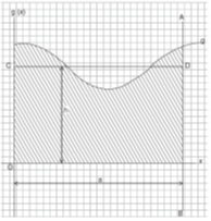0] p. : 205-6

[viii] “The process of computing probabilities often depends on being able to count, in the usual sense of counting, “1, 2, 3,” and so on. The usual way of counting becomes quite tedious in some complicated situations” [11] p. 5-6.

The probability theory foundation rests on counting unique and non-overlapping units/entities, or events. The logical operations involved in the very definitions of conditional and joint probabilities require distinguishability, when one e.g. talks about P(AB) and P(A | B): events A and B happening means A, and ‘then’ B happening, separately, distinctly: but ‘then’ here encodes simultaneity, for is time passes, we have complications, one being that the ‘independence’ is not a symmetric relation anymore. But see “Sometimes the notions of independent events and mutually exclusive events are confused with each other, because both notions give the impression that “the two events do not have anything to do with each other.” The property of independence depends not only on the two events being considered but also on the particular probability function defined on the sample space. It is possible for P(AB) and P(A)P(B) to be equal to each other with one set of probabilities and to be unequal with another set of probabilities. But see: “mutually exclusive” simply means the two events have no points in common, and no matter what probability function is defined on the sample space, AB is empty, so P(AB) = 0. If A and B are mutually exclusive, they will be independent only if either P(A) or P(B) equals zero, since Equation 5 must be satisfied.” [11] P. 19

[ix] ‘Same’ and ‘different’ can run into ontological troubles when ‘small’ and ‘large’ infinity are added in the arguments: a tricycle is indistinguishable from the same object in which one removes an infinitesimally small ‘chunk’, say part of the ‘third’ wheel, and so one after removing a 2^nd such small part: if we continue this process until the 3^rd wheel is completely removed, we arrive at a bicycle, which has a different ontological status, but each intermediate steps were indistinguishable entities. A good visual depiction of the challenge is the ‘turning of a square into a circle’. Another exercise applies to removing neurons from a human brain 1 by 1, and replacing them with electronic counterparts: at what point the entity becomes a ‘machine’?

* Another complication is the ‘decomposition’ statistical habit: we divide up the variance into 2 (mutually exclusive, we assume, hence additive) components, like: “The total variance in a phenotypic trait in a population can be divided into two types, between-genotype-variance and within-genotype-variance. Some phenotypic differences in a population are due to genotypic differences; this variance, the between-genotype-variance, is represented by V_G‘ The remaining variance, obviously, is not due to genotypic differences. The name given this type of variance is environmental variance, V_e. 4 Thus we have the following equation (where V_T‘ stands for the total variance): 5 V_T = V_G + V_e (3) [This equation and what follows in the genetic definition of heritability require some strong assumptions. See Roughgarden ([12] 1979, chapter 9) for details.]” [13], p. 60