General definitional and notational setup
*** Causality is not directly detectable or observable, much like forces[i] or energy aren’t either: it needs to be discovered/uncovered – ‘detected’ through observational consequences[ii]; on the other hand, it’s a pretty natural intuitive human notion[iii], yet is considered a worthy ‘problem’[iv].
*** Causality is hardly a statistical matter, and it shows up at the very roots of scientific inquiries: the basic notions of substance and time, e.g. are defined in excessive proximity to causal relations: e.g. abstract entities (like ‘number 7’) are those that cannot cause anything[v], unlike ‘concrete substances’, and time itself has definitions overlapping with causality [2-6].
*** Causal language[vi] differs drastically by scientific field[vii], and some are more shy than others in using the “C” word. In statistics it has been kept at bay for many decades, and epidemiologists have been to first advocates among statisticians at large (Tyler VanderWeele, e.g., but also Jay Kaufman [8] and [9] in health disparities, and many other nowadays).
+++ This follows my ‘let’s talk (just talk!, no math!) about causality’ recent philosophy. The old adagio “correlation does not imply causation” is a structural misunderstanding of constructs: while each are a 2-objects relation, causation is not symmetric, as correlation is, and ‘proceeding from one to the other’ requires more than the 2 objects of interest. The simple solution was offered >100 years ago by Sewall Wright, and I rephrase to modern language: “a correlation can come from: either variable causing the other one, or another variable causing both”. This makes clear the ‘logical tension’ and the proper solution: we need to step above the 2 ingredients to make causal statements (otherwise we might just reply: “correlation implies causation, but only sometimes”, when there is a causal component of the relation in there).
To rephrase still: causal inference involves decomposing correlations into their causal and non-causal components. Simple, right? Incidentally, a parallel view uses a similar decomposition maneuver. [0]
*** Even ‘simple’ questions like ‘What causes the universe to expand?’ rely on deeply unobservable constructs, like dark energy.[viii]
*** In medicine, causal questions are broadly aimed at ‘changing the current course of events’[ix] in the future, whereas in astronomy e.g. mere deep descriptive understanding of ‘how things work’ is a goal in itself: finding the laws governing the Universe.[x]
*** The task then is to discover “which variable ‘listens to’ which others“ (‘Book of Why’ BoW p. 7), e.g. whether blood glucose (say measured by hemoglobin A1c) ‘listens to’ one’s body weight (say measured by body mass index, BMI), and responds to it: this metaphor invites deeper delving into how the ‘listening’ works[xi]: is an asteroid ‘listening’ to the Earth’s gravity when heading to it? Does it have a choice not to listen, like biological bodies do? Since biological entities are the first ones to collect information and use it in choosing to respond differently, to benefit themselves, the ‘listening’ appears to make less sense before the first living organisms appeared: all natural bodies and substances before that blindly (and strictly, without choice) followed the tight grip of the natural laws, gravity among them being the central one.[xii]
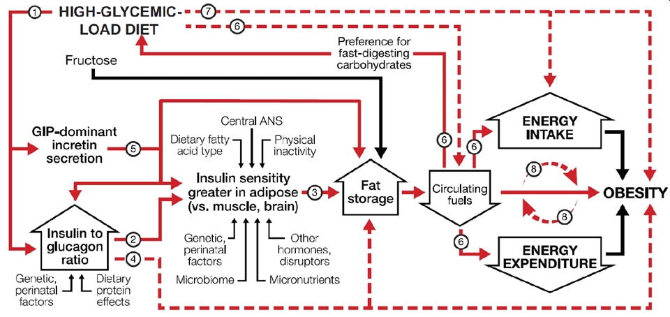
*** Note that the way BMI relates to A1c is not merely direct and linear, e.g. [48]:
FIGURE 1 Dynamic phase of obesity development in the carbohydrate-insulin model[xiii].
*** Intuitively grasping how causal effects are ‘extracted’ from correlational-kind data, a bit of notational setup will be decisive: for the A1c(BMI) relation of interest, or BMI -> A1c, or probability(A1c | BMI), where “|” stands for ‘given’, we want to find out whether lowering BMI would cause a A1c drop, and then by how much. To answer the ‘cause-effect’ research question (RQ), we simply need to compare for each patient i his/her A1c’s under the current (present state) CurrentBMI vs. a ‘what if’ potential state If.LowerBMI:
A1c i CurrentBMI vs. A1c i If.LowerBMI
or with classic ‘treatment’ (Tx) as the cause: A1c i If.Treated vs. A1c i If.NotTreated
where superscripts mean ‘it could happen up there’ [xiv] A1c i If.LowerBMI , vs. what actually happened ‘here on the ground’, in this reality A1c i CurrentBMI. More details in the footnote, suffice to say that there is a causal effect of BMI on A1c for patient i if: A1c i If.LowerBMI ≠ A1c i CurrentBMI! One of these two quantities however can never be ‘seen’, once reality kicks in: either one has his/her current BMI, or a lower BMI!
Note though that when realized, potential values come ‘down here on the ground’ (become visible):
A1c i *If.NotTreated NotTreated = A1c i NotTreated and
A1c i *If.Treated Treated = A1c i Treated
in which I added the *, for ‘never visible’: what would have happened to these folks, but… didn’t (couldn’t)! The fundamental causal inference problem is that one of these 2 in each condition is ‘missing’:
A1c i *If.Treated NotTreated & A1c i *If.NotTreated Treated
***The statistical trickery to still derive a causal effect from such ‘observational’ data (i.e. not from a randomized controlled research design) is to ‘identify’ the average causal effect among those who say lowered their BMI, Average(A1c i If.LowerBMI LoweredBMI – A1c i *If.SameBMI LoweredBMI), in which we added the *, for ‘never visible’: what would have happened to these folks, but… didn’t!
We do this by ‘wiping off’ a bias quantity, the ‘selection bias’[xv]. All this math is drastically simplified if one uses Judea Pearl’s notation for ‘setting’ the predictor to a value, so Average(A1c i If.LowerBMI) becomes simply Average(A1c i | (set (BMI=Lower))[xvi], [55, 56], where “set” symbolizes an actual intervention that sets to BMI to a lower value, and E means ‘expected (average) value of’: the challenge of ‘causal inference’ then is ‘simply’ deriving the causal quantity Average(A1c | (set (BMI=Lower)) from the observational one Average(A1c | ‘seeing’ BMI=Lower). Observing BMI=Low is NOT the same as ‘setting’ it to ‘Low’, or ‘intervening’ to ‘do’ that:
Average(A1c i | ‘see’ BMI=Lower) ≠ Average(A1c i | ‘set’ BMI=Lower)
or Average(A1c i | ‘see’ BMI=Lower) ≠ Average(A1c i | ‘do’ BMI=Lower)
***Again, statistics can ‘recover’ the causal effects from observational (non-interventional) data when it can turn all ‘set’ (or ‘do’) into ‘see’ in the formulas: then, the math (or software, or AI) can directly yield the actual causal effect: even a simple t-test or a chi-squared test would thus become a ‘causal analysis’.
*** I start with an illustration of the simplest ‘data’, the yes/no, presence/absence, or 1/0, like diabetic/not (which can carry some error in it too[xvii]). This is a quick overview of several topics that all rely on this simplest possible data setup: a 2by2 binary fields/variables, all using the simple 4-cell setup (0,0), (1,0), (0,1), and (1,1). They make use of the information derived from such a setup completely differently:
***.1. Finding ‘it’ vs. missing ‘it’: the medical sensitivity vs. specificity (& ROC curve – to be added)
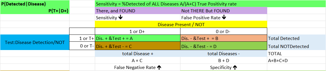
The setup here is slightly different than most 2by2 tables(as chi-squared test examples, e.g.), and it has Test(for a disease), on the left, and Disease, on top, and inside: (1,1) (1,0), first row, then (0,1), (0,0), or the a,b,c, and d, as they are better known (an image is shown). They mean sequentially:
a (1,1) Test is positive, Disease present, so we have (+,+) = Good!
b (1,0),Test is positive, Disease not there, so (+,-) = Bad! first row, then
c (0,1), Test is negative, Disease present, so (-,+) = Bad!
d (0,0), Test is negative, Disease not there, so (-,-) = Good!
Sensitivity reads the 1st column downwards: n(1,1) / [n(1,1) + n(0,1)] or with | meaning ‘given’
P(Test + | Disease +) – this has a more intuitive write-up: percent of all disease+ patients with test+
Specificity reads the 2nd column upwards: n(0,0) / [n(0,0) + n(1,0)] or
P(Test – | Disease -) : percent of all disease- patients with test-
*** Note that it is different to talk about P(Disease + | Test +), than about P(Test + | Disease +), which has a more natural direction; the ‘direction’ differs: we ‘condition on‘ (know) one, or the other.
*** Note that this 2×2 setup is not direction-less[xviii], yet here the 1st # talks about the LEFT label (test), second about the TOP label (disease, so (1, 0) means (Test + , Disease -); 2by2 tables read more naturally from left->right and top-down. However, sensitivity and specificity read P(Test | Disease), so the ‘given’ (or ‘knowing’) is the Disease, which ‘happens first. This setup becomes more meaningful when time is incorporated, as in RQ.2. in part 2, which has the before & after of a binary category: here P(Post | Pre) makes sense, but P(Pre | Post) does not.
*** A similar setup is the by-product of a logistic regression analysis, when the predictors of a binary outcome are more/less useful in ‘correctly’ assigning 1’s and 0’s to their category; the ‘classification table’ shows the correct assignments (1,1) & (0,0), and the incorrect ones (1,0), (0,1), and provide an average of percent cases incorrectly classified.
***2. In formal logic “If Premise – Then Conclusion” or simply “Premise -> Conclusion” follows formal rules, which simply say that the entire statement “Premise -> Conclusion” is false in relation to the 2 ingredients truth value only in 1 circumstance: When “True -> False”: truth cannot lead to falsehood! A peculiar one however is “False -> True”, this whole statement is ‘True’, (along with the other 2 possibilities “True -> True” and “False -> False”), because, as Claude.ai says “Since the condition is never met, the implication can’t be falsified.”, meaning because we start in an ‘impossible world’, we cannot test its truth value… “If pigs could fly, then anything goes” pretty much…
If we follow the four-cell setup known in the sensitivity/specificity context below (1,1) (1,0), (0,1), (0,0), the ‘first’ is logically the ‘If’ (vertical, from up to down, column), the second the ‘Then’ (horizontal, left to right, row) follow
a (1,1), IF is True, THEN is True too, so we have (+,+) or
b (1,0), IF is True, THEN is False, so (+,-) : this argument only of the 4 is FALSE
c (0,1), IF is False, THEN is True, so (-,+)
d (0,0), IF is False, THEN is False too, so (-,-)
***.3. H0 (null hypothesis) vs. H1 and what statistics says: rejecting H0 – seeing ‘the effect’ vs. not; unfortunately, the Null Hypothesis language leads to double (and more) negations (fail to reject H0… meaning “we see no effect), so the following emphasizes the ‘Effect seeing’ (or not) phrasing.
If we follow the same four-cell setup known in the sensitivity/specificity context below (1,1) (1,0), (0,1), (0,0), the ‘first’ category is logically ‘there is/not an Effect’ (= ‘H0 (null hypothesis) if true/false’, vertical, from up to down, column), the second the ‘Statistics finds/not an effect’ (= ‘we reject/fail to reject H0 t, horizontal, left to right, row) follow
a: (1,1) or (+ | +): There is an Effect (H0=False), and Statistics finds it (rejects H0 true too); we correctly say ‘There IS an Effect’! This is (1-β) = ‘statistical power’ that we often we need estimated before a study is started: we want some solid/large value here, a good likelihood we will FIND and Effect when it’s there! This is ~= (akin to) the SENSITIVITY of a test, from above!
b: (1,0) or (+ | -): There is NO Effect (H0=True), and Statistics finds it (rejects H0 true); = we make a Type I error: “True null hypothesis is incorrectly rejected”; Type I because it is most serious, we ‘find something that doesn’t exist’ (i.e. ‘make up stuff’)! This is α, the customary .05 (5%) threshold value: we set this upfront, to as small an uncertainty value as we are willing to tolerate.
c: (0,1) or (- | +): There is an Effect (H0=False), BUT Statistics does NOT find it (‘we fail to reject’ H0); we make a make a Type II error: “true null hypothesis is incorrectly rejected” This is β.
d: (0,0) or (- | -): There is NO Effect (H0=True), and Statistics does NOT find it either: we correctly say ‘There if NO effect’! This is(1-α).
***It is advisable to set up expectations based on prior knowledge in the form of a Hypothesis: Overweight -> Diabetes, (a causal statement), or a RQ: “Overweight -> Diabetes?”. The hypothesis testing procedure is a flexibly ‘sharp’ decision process, can be e.g. 2-sigma’, rejecting H0 based on the ‘2 standard errors away’ criterion (‘p < .05’), common in medicine and health research, or more conservatively based on the 5-sigma rule in physics (‘p < .00006’): the = .05 rule is a ‘rule of thumb’, but thumbs differ widely in size…
***I will demonstrate in part 2 several statistical tests and analyses, with an emphasis on the mechanics of each, the ‘how to’, all of them done ‘by hand’ and in Excel alone (no ‘sophisticated’ statistical software needed).
FOOTnotes:
Judea Pearl said in his ‘Book of Why’ (ch.1 here; books seems to be online here): “Flip two coins simultaneously one hundred times and write down the results only when at least one of them comes up heads. Looking at your table, which will probably contain roughly seventy-five entries, you will see that the outcomes of the two simultaneous coin flips are not independent. Every time Coin 1 landed tails, Coin 2 landed heads. How is this possible? Did the coins somehow communicate with each other at light speed? Of course not. In reality you conditioned on a collider by censoring all the tails-tails outcomes. “Why:202)
The format of the book does not allow ‘spelling out’ of every detail… (some readers reported this too), so I will try. This becomes ‘visible’ when one ‘does’ it (! a ‘do’ operation…), say in Excel/GSheets directly. I will explain it ‘verbally’ (a separate post will walk through the Excel exercise). So:
If one generates a series or random yes/no (1/0) events, say flipping a coin 100 times: we list the results in a 1st column; repeat this process, list results in a 2nd column: the 2 cannot be correlated: they are both random occurrences. A third column can be built off the first two, by coding 0 when both ingredients were 0, and 1 otherwise (which is: 3rd = 1st+2nd−1st∙2nd): this 3rd is ‘determined’ causally (or ‘caused deterministically’…) by the first 2. What one can verify directly is:
- Regressing 2nd on 1st will yield a null (near-zero, statistically) relation always (nearly so); BUT, controlling for the 3rd will always yield a non-null (conditional) relation: this is the artificial ‘creation’ of a correlation between two predictors of the same outcome, when conditioning on that outcome: THIS is the collider problem!
- Following the example as phrased in the book, but now giving extra-meaning to the 1st and the 2nd: say 1st is head injuries and 2nd is heart ‘problems’ (as a symptom, palpitations of a more serious nature, e.g., that would make one go to the hospital): these 2 should not relate for any natural reason, but if we restrict our data collection to those who had either, by selecting data from a hospital database, all of a sudden we will see a correlation between them. Granted, this particular one will be negative, patients in the hospital either have one, and not the other one (and vice versa). This is pretty much almost any medical study… which excludes healthy folks, because… there is ‘nothing to see there’.
– There are other implications to be aware of: depending on the sign of the two effects between 1st and 2nd, and the 3rd, this ‘artifact’ can be >0 or <0: this has the consequence of ‘shifting’ the ‘Null’ point of our hypothesis testing process, technically. We start off ‘crooked’, and we should correct for this!
+++ “we can decompose the observed outcome of a treatment into two effects:
Outcome for treated −Outcome for untreated
= (Outcome for treated −Outcome for treated if not treated) +
+ (Outcome for treated if not treated− Outcome for untreated) =
= Impact of treatment on treated + selection bias.” {Varian, 2016 #15819} p. 7311
[i] “What are the merits of these fictitious variables called causes that make them worthy of such relentless human pursuit, and what makes causal explanations so pleasing and comforting once they are found? We take the position that human obsession with causation, like many other psychological compulsions, is computationally motivated. Causal models are attractive mainly because they provide effective data structures for representing empirical knowledge-they can be queried and updated at high speed with minimal external supervision. The effectiveness of causal models stems from their modular architecture, i.e., an architecture in which dependencies among variables are mediated by a few central mechanisms. “ p. 383 ‘ 8. Learning Structure from Data\ 8.1. Causality, Modularity, and Tree Structures’; “the construct of causality is merely a tentative, expedient device for encoding complex structures of dependencies in the closed world of a predefined set of variables. It serves to highlight useful independencies at a given level of abstraction, but causal relationships undergo drastic change upon the introduction of new variables.” P. 397
“With its dual role, summarizing and decomposing, a causal variable is analogous to an orchestra conductor: It achieves coordinated behavior through central communication and thereby relieves the players of having to communicate directly with one another. In the physical sciences, a classic example of such coordination is afield (e.g., gravitational, electric, or magnetic). Although there is a one-to-one mathematical correspondence between the electric field and the electric charges in terms of which it is defined, nearly every physicist takes the next step and ascribes physical reality to the electric field, imagining that in every point of space there is some real physical phenomenon taking place which determines both the magnitude and direction assigned to that point. This psychological construct had a huge impact on the historical development of electrical science. It decomposed the complex phenomena associated with interacting electrical charges into two independent processes: The creation of the field at a given point by the surrounding charges and the conversion of the field into a physical force once another charge passes near that point.” {Pearl, 1988 #5884} P. 384
[ii] “An interesting philosophical question is whether any method based on probabilities can identify causal directionality among observable variables.” {Pearl, 1988 #5884} p. 396, Learning Structure from Data “Formally speaking, probabilistic analysis is indeed sensitive only to covariations, so it can never distinguish genuine causal dependencies from spurious correlations, i.e., variations coordinated by some common, often unknown causal mechanism. But what is the operational meaning of a genuine causal influence? How do humans distinguish it from spurious correlation? Our instinct is to invoke the notion of control; e.g., we can cause the ice to melt by lighting a fire but we cannot cause fire by melting the ice. Yet the element of control is often missing from causal schemas. For example, we say that the rain caused the grass to become wet despite our being unable to control the rain. The only way to tell that wet grass does not cause rain is to find some other means of getting the grass wet, clearly distinct from rain, and to verify that when the other means is activated, the ground surely gets wet while the rain refuses to fall. Thus, the perception of voluntary control is in itself merely a by-product of covariation observed on a larger set of variables [Simon 1980], including, for example, the mechanism of turning one’s sprinkler on. In other words, whether X causes Y or Y causes X is not something that can be determined by running experiments on the pair (X, Y), in isolation from the rest of the world. The test for causal directionality must involve at least one additional variable, say Z, to test if by activating Z we can create variations in Y and none in X, or alternatively, if variations in Z are accompanied by variations in X while Y remains unaltered. This is exactly the meaning of causality that the polytree recovery algorithm attributes to the arrows on the branches. The meaning relates not to a single branch in isolation but to an assembly of branches heading toward a single node. An arrow is drawn from X to Y and not the other way around when a variable Z is found that correlates with Y but not with X (see Figure 8.2a). The discovery of the third variable Z, however, does not necessarily mean that X and Z are the ultimate causes of Y. The relationship among the three could change entirely upon the discovery of new variables.” p. 396-7
[iii] “After all, if you and I share the same understanding of physics, you should be able to figure out for yourself which mechanism it is that must be perturbed in order to realize the specified new event, and this should enable you to predict the rest of the scenario.
This linguistic abbreviation defines a new relation among events, a relation we normally call “causation”: Event A causes B, if the perturbation needed for realizing A entails the realization of B.2 (2 The word “needed” connotes minimality and can be translated to: ” .. .if every minimal perturbation realizing A, entails B”.) ” {Pearl, 1997 #15498} p. 55
[iv] “When we ask, for example, what causes this fire, it is not its being this but its being fire that we are seeking to account for.” {Anderson, 1938 #15495} p. 128
[v] “I shall understand by a ‘substance’ a particular thing, capable of causing or being caused, such as Richard Swinburne, or a particular table, or a particular electron, or the planet Venus.” [1] Drive
[vi] “Despite heroic efforts by the geneticist Sewall Wright (1889–1988), causal vocabulary was virtually prohibited for more than half a century. And when you prohibit speech, you prohibit thought and stifle principles, methods, and tools” Pearl’s BoW p. 5.
[vii] What ‘scientific research’ is requires a long detour; a simpler approach is to delineate from ‘non-scientific’ research, which some deem to be the ‘farthest away’, e.g. theology, philosophy or knowledge through art [7] (it is rather paradoxical to consider philosophy non-scientific, as long as it provides all sciences the main argumentation tool, formal logic).
[viii] And this only talks about the ‘observable’ Universe, which is to the entire Universe like an atom is to the observable Universe…
[ix] “This chapter deals with the problem of con-structing a network automatically from direct empirical observations, thus bypassing the human link in the process known as knowledge acquisition. […] it is more convenient to execute the learning process in two separate phases: structure learning and parameter learning. [ …] Our focus in this chapter will be on learning structures rather than parameters. […] e shall focus on causal structures and in particular on causal trees and polytrees, where the computational role of causality as a modularizer of knowledge achieves its fullest realization. “ & “Causal labeling creates modularity not only by separating the past from the future, but also by decoupling events occurring at the same time. Knowing the set of immediate causes ПB renders X independent of all other variables except X’s descendant; many of these variables may occur at the same time as X, or even later. In fact, this sort of independence is causality’s most universal and distinctive characteristic. In medical diagnosis, for example, a group of co-occurring symptoms often become independent of each other once we identify the disease that caused them. When some of the symptoms directly influence each other, the medical profession invents a name for that interaction (e.g., syndrome, complication, or clinical state) and treats it as a new auxiliary variable, which again assumes the modularization role characteristic of causal agents-knowing the state of the auxiliary variable renders the interacting symptoms independent of each other.” {Pearl, 1988 #5884} p. 385 ‘8. Learning Structure from Data\ 8.1. Causality, Modularity, and Tree Structures’;
[x] The graphical causal models in medicine are gaining ground: [10] [11] [12] [12-33] [11, 27, 34-45]
[xi] “The calculus of causation consists of two languages: causal diagrams, to express what we know, and a symbolic language, resembling algebra, to express what we want to know. The causal diagrams are simply dot-and-arrow pictures that summarize our existing scientific knowledge. The dots represent quantities of interest, called “variables,” and the arrows represent known or suspected causal relationships between those variables—namely, which variable “listens” to which others. “ BoW [46], p. 7
[xii] Listening from a communication (science) standpoint is also an active and deliberate process, not a mere ‘reception of data’, but a meaning-seeking activity (‘sensemaking’ is another such label, see e.g. in the AI context [47]). Note that a large part of the causality thinking in the 1980’s happened on what was then labeled AI research, or ‘device behavior’ {Iwasaki, 1986 #15488}, and in ‘decision science’, see e.g. {Gärdenfors, 2003 #15502} or {Georgeff, 1988 #15503}.
[xiii] “The relation of energy intake and expenditure to obesity is congruent with the conventional model. However, these components of energy balance are proximate, not root, causes of weight gain. In the compensatory phase (not depicted), insulin resistance increases, and weight gain slows, as circulating fuel concentration rises. (Circulating fuels, as measured in blood, are a proxy for fuel sensing and substrate oxidation in key organs.) Other hormones with effects on adipocytes include sex steroids and cortisol. Fructose may promote hepatic de novo lipogenesis and affect intestinal function, among other actions, through mechanisms independent of, and synergistic with, glucose. Solid red arrows indicate sequential steps in the central causal pathway; associated numbers indicate testable hypotheses as considered in the text. Interrupted red arrows and associated numbers indicate testable hypotheses comprising multiple causal steps. Black arrows indicate other relations. ANS, autonomic nervous system; GIP, glucose-dependent insulinotropic peptide.” Medical diagnosing has been the focus or early ‘decision science’ works, see the ‘Causal Understanding’ [49] figure e.g.
[xiv] This notation was also used by [50] and by [51] p. 244, and by Lok [52]; Reichenbach also used a close-by symbol : “where the events that show a slight variation [from E] are designated by E*:” p.137 [53].
[xv] The process is more detailed: we subtract and add one same term to the causal effect, and then ‘take expectations’, i.e. averages the quantities across patients:
E(CausalEffecti) = E (A1ciIf.LowerBMI LoweredBMI – A1ciIf.CurrentBMI Current.BMI) =
E (A1ciIf.LowerBMI LoweredBMI – A1c*iIf.CurrentBMI LoweredBMI ) + E (A1c*iIf.CurrentBMI LoweredBMI – A1ciIf.CurrentBMI Current.BMI) =
ATT + Selection.Bias
Where ATT = the average treatment effect on the treated: how much the A1c would … not drop among those who did lower their BMI, if… they didn’t! Note, Eric Brunner from UConn stated it using econometric language and labels (𝐷 is Treatment) : “We suspect we won’t be able to learn about the causal effect of college education simply by comparing the average levels of earnings by education status because of selection bias:
𝐸[𝑌𝑖|𝐷𝑖=1]−𝐸[𝑌𝑖|𝐷𝑖=0]= 𝐸[𝑌1𝑖|𝐷𝑖=1]−𝐸[𝑌0𝑖|𝐷𝑖=1] (ATT)
+𝐸[𝑌0𝑖|𝐷𝑖=1]−𝐸[𝑌0𝑖|𝐷𝑖=0] (Selection bias). We suspect that potential outcomes under non-college status are better for those that went to college than for those that did not; i.e. there is positive selection bias” in his ‘Causal Evaluation’ graduate course handout]; an alternative notation brings both real&potential worlds in one formula, see Jordi Vallverdú’s book (but common among causality writers) ‘Causality for Artificial Intelligence. From a Philosophical Perspective’: “Let Y(T) represent the potential outcome for a patient with treatment assignment Y (where T is either 0 or 1). We can express the observed outcome Y as follows:
Y = T × Y(1) + (1 – T) × Y(0)” or with my ‘re-labeling’, similar to David A. Freedman‘s in fact (Yi = XiYiT + (1 − Xi)YiC :
YRealized = T × YIf.(T=1) + (1 – T) × YIf(T=0)
[xvi] We use Average for better intuition; mathematically inclined analysts use instead E(A1c), for ‘expectation’, which is the proper way to define a ‘typical patient’s value’, or the mean of a variable. For a variable X with discrete values, the mean is μX = E(X) = Σi [xi·p(xi)], while for one with continuous values μX = E(X) = ([54], p. 152).
[xvii] Even presence vs. absence can be sometimes difficult to separate: “Whoever studied newspapers in the last decades came across the difficulties of defining when a person is dead, allowing the organs to be transplanted. Our hair and nails still grow long after our hearts stop beating;” [57] p. 2. This topic of measurement error of binary measures is rarely talked about, in psychometric sense.
[xviii] The confounding of ‘causality’ and ‘time’ is a known definitional problem: e.g. VanFraasen cites Reichenbach defining time in terms of causality ([58], p, 190), and many define time on the basis of the time construct.
*** Reichenbach himself said e.g. “we must now make sure that our definition of “later than” does not involve circular reasoning. Can we actually recognize what is a cause and what is an effect without knowing their temporal order?
Should we not argue, rather, that of two causally connected events the effect is the later one?
This objection proceeds from the assumption that causality indicates a connection between two events, but does not assign a direction to them. This assumption, however, is erroneous. Causality establishes not a symmetrical but an asymmetrical relation between two events.
If we represent the cause-effect relation by the symbol C, the two cases C(E1, E2) and C(E2, E1) can be distinguished; experience tells us which of the two cases actually occurs. We can state this distinction as follows:
If E1 is the cause of E2. then a small variation (a mark)” in E1 is associated with a small variation in E2. whereas small variations in E2 are not associated with variations in E1.” [53] P. 136
References
- Swinburne, R., The coherence of theism. 2016: Oxford University Press.
- Hall, E.W., Time and Causality. The Philosophical Review, 1934. 43(4): p. 333-350.
- Davidson, R., Time and Causality. Annals of Economics and Statistics, 2013(109/110): p. 7-22.
- Buehner, M.J., Time and causality. 2014, Frontiers Media SA. p. 228.
- Kleinberg, S., Causality, probability, and time. 2013: Cambridge University Press.
- Swinburne, R., Space, Time and Causality. 1983.
- David, D.O., Metodologia cercetării clinice: fundamente. 2006: Polirom.
- Kaufman, J.S. and S. Kaufman, Assessment of Structured Socioeconomic Effects on Health. Epidemiology, 2001. 12(2): p. 157-167.
- Kaufman, J.S. and R.S. Cooper, Seeking causal explanations in social epidemiology. American journal of epidemiology, 1999. 150(2): p. 113-120.
- Caniglia, E.C., et al., Does Reducing Drinking in Patients with Unhealthy Alcohol Use Improve Pain Interference, Use of Other Substances, and Psychiatric Symptoms? Alcoholism: Clinical and Experimental Research, 2020. n/a(n/a).
- Pearce, N. and D.A. Lawlor, Causal inference—so much more than statistics. International journal of epidemiology, 2016. 45(6): p. 1895-1903.
- Staplin, N., et al., Use of causal diagrams to inform the design and interpretation of observational studies: an example from the Study of Heart and Renal Protection (SHARP). Clinical Journal of the American Society of Nephrology, 2017. 12(3): p. 546-552.
- Burden, A.F. and N. Timpson, Ethnicity, heart failure, atrial fibrillation and diabetes: collider bias. 2019, BMJ Publishing Group Ltd and British Cardiovascular Society.
- Lamprea-Montealegre, J.A., et al., Apolipoprotein B, Triglyceride-Rich Lipoproteins, and Risk of Cardiovascular Events in Persons with CKD. Clinical Journal of the American Society of Nephrology, 2020. 15(1): p. 47-60.
- Vo, T.-T., et al., The conduct and reporting of mediation analysis in recently published randomized controlled trials: results from a methodological systematic review. Journal of clinical epidemiology, 2020. 117: p. 78-88.
- Fotheringham, J., et al., The association between longer haemodialysis treatment times and hospitalization and mortality after the two-day break in individuals receiving three times a week haemodialysis. Nephrology Dialysis Transplantation, 2019. 34(9): p. 1577-1584.
- Jhee, J.H., et al., Secondhand smoke and CKD. Clinical Journal of the American Society of Nephrology, 2019. 14(4): p. 515-522.
- Woods, G.N., et al., Chronic kidney disease is associated with greater bone marrow adiposity. Journal of Bone and Mineral Research, 2018. 33(12): p. 2158-2164.
- Storey, B.C., et al., Lowering LDL cholesterol reduces cardiovascular risk independently of presence of inflammation. Kidney international, 2018. 93(4): p. 1000-1007.
- Waikar, S.S., et al., Association of urinary oxalate excretion with the risk of chronic kidney disease progression. JAMA internal medicine, 2019. 179(4): p. 542-551.
- Watkins, T.R., Understanding uncertainty and bias to improve causal inference in health intervention research https://ses.library.usyd.edu.au/bitstream/handle/2123/20772/watkins_tr_thesis.pdf. 2018.
- Bjornstad, E.C., et al., Racial and health insurance disparities in pediatric acute kidney injury in the USA. Pediatric Nephrology, 2020: p. 1-12.
- Leite, T.T., et al., Respiratory parameters and acute kidney injury in acute respiratory distress syndrome: a causal inference study. Annals of Translational Medicine, 2019. 7(23).
- Groenwold, R.H., T.M. Palmer, and K. Tilling, Conditioning on a mediator to adjust for unmeasured confounding https://osf.io/sj7ch/. 2019.
- Tørnes, M., et al., Hospital-Level Variations in Rates of Inpatient Urinary Tract Infections in Stroke. Frontiers in neurology, 2019. 10: p. 827.
- Benedum, C.M., Applications of big data approaches to topics in infectious disease epidemiology. 2019, Boston University Available from ProQuest 2241610916.
- Gaskell, A.L. and J.W. Sleigh, An Introduction to Causal Diagrams for Anesthesiology Research. Anesthesiology: The Journal of the American Society of Anesthesiologists, 2020. 132(5): p. 951-967.
- Fotheringham, J., et al., Hospitalization and mortality following non-attendance for hemodialysis according to dialysis day of the week: a European cohort study. BMC Nephrology, 2020. 21(1): p. 1-10.
- Sawchik, J., J. Hamdani, and M. Vanhaeverbeek, Randomized clinical trials and observational studies in the assessment of drug safety. Revue d’epidemiologie et de sante publique, 2018. 66(3): p. 217-225.
- Banack, H.R., et al., Investigating and Remediating Selection Bias in Geriatrics Research: The Selection Bias Toolkit. Journal of the American Geriatrics Society, 2019. 67(9): p. 1970-1976.
- Tørnes, M., et al., Does service heterogeneity have an impact on acute hospital length of stay in stroke? A UK-based multicentre prospective cohort study. BMJ open, 2019. 9(4): p. e024506.
- Ferguson, T.W. and N. Tangri, Identifying Potential Biases in the Nephrology Literature. Advances in Chronic Kidney Disease, 2016. 23(6): p. 373-376.
- Zeraatkar, D., et al., Methods for the Selection of Covariates in Nutritional Epidemiology Studies: A Meta-Epidemiological Review. Current developments in nutrition, 2019. 3(10): p. nzz104.
- Birungi, N., et al., Assessing causal effects of early life‐course factors on early childhood caries in 5‐year‐old Ugandan children using directed acyclic graphs (DAG s): A prospective cohort study. Community Dentistry and Oral Epidemiology, 2017. 45(6): p. 512-521.
- Henckel, L., E. Perković, and M.H. Maathuis, Graphical criteria for efficient total effect estimation via adjustment in causal linear models. arXiv preprint arXiv:1907.02435, 2019.
- Sourial, N., et al., Testing group differences for confounder selection in nonrandomized studies: flawed practice. Canadian Medical Association Journal, 2019. 191(43): p. E1189-E1193.
- Shapiro, D.D. and P. Msaouel, Causal Diagram Techniques for Urologic Oncology Research. Clinical Genitourinary Cancer, 2020.
- Hancox, R.J., When is a confounder not a confounder? Respirology, 2019. 24(2): p. 105-106.
- Kuehne, F., et al., Guidance for a causal comparative effectiveness analysis emulating a target trial based on big real world evidence: when to start statin treatment. Journal of comparative effectiveness research, 2019. 8(12): p. 1013-1025.
- Etminan, M., G.S. Collins, and M.A. Mansournia, Using causal diagrams to improve the design and interpretation of medical research. Chest, 2020. 158(1): p. S21-S28.
- Oates, C.J., et al., Repair of partly misspecified causal diagrams. Epidemiology, 2017. 28(4): p. 548-552.
- Wang, T., et al., Sensitivity analysis for mistakenly adjusting for mediators in estimating total effect in observational studies. BMJ open, 2017. 7(11).
- Andreano, A., et al., Adherence to guidelines and breast cancer patients survival: a population-based cohort study analyzed with a causal inference approach. Breast Cancer Research and Treatment, 2017. 164(1): p. 119-131.
- Lederer, D.J., et al., Control of confounding and reporting of results in causal inference studies. Guidance for authors from editors of respiratory, sleep, and critical care journals. Annals of the American Thoracic Society, 2019. 16(1): p. 22-28.
- Williamson, E.J., et al., Introduction to causal diagrams for confounder selection. Respirology, 2014. 19(3): p. 303-311.
- Pearl, J. and D. Mackenzie, The Book of Why: The New Science of Cause and Effect. 2018, London, UK: Basic Books, Penguin Books Limited.
- Madsbjerg, C., Sensemaking: The Power of the Humanities in the Age of the Algorithm. 2017: Grand Central Publishing.
- Ludwig, D.S., et al., The carbohydrate-insulin model: a physiological perspective on the obesity pandemic. The American Journal of Clinical Nutrition, 2021.
- Patil, R., P. Szolovitz, and W. Schwartz. Causal understanding of patient illness in patient diagnosis. in Proceedings of AAAI-82. 1982.
- Joffe, M.M., W.P. Yang, and H.I. Feldman, Selective ignorability assumptions in causal inference. The International Journal of Biostatistics, 2010. 6(2).
- Kohler, U. and F. Kreuter, Data analysis using Stata. 3 ed. 2012: Stata press.
- Lok, J.J. and R.J. Bosch, Causal organic indirect and direct effects: Closer to the original approach to mediation analysis, with a product method for binary mediators. Epidemiology, 2021. 32(3): p. 412-420.
- Reichenbach, H., The philosophy of space and time. 1957: Courier Corporation.
- Devore, J.L., Probability and statistics for Engineering and the Sciences. Pacific Grove: Brooks/Cole, 2016.
- Pearl, J. On the Statistical Interpretation of Structural Equations. UCLA Cognitive Systems Laboratory, Technical Report (R-200), 2011.
- Pearl, J., [Bayesian Analysis in Expert Systems]: Comment: Graphical Models, Causality and Intervention. Statistical Science, 1993. 8(3): p. 266-269.
- Stauffer, D., Introduction to statistical physics outside physics. Physica A: Statistical Mechanics and Its Applications, 2004. 336(1-2): p. 1-5.
- Van Fraassen, B.C., An introduction to the philosophy of time and space. 1970.
- Varian, H. R. (2016). Causal inference in economics and marketing. Proceedings of the National Academy of Sciences, 113(27), 7310-7315.